Output files

When BowshockPy is run from the terminal using an input file, it will create the path models/<modelname> if it does not exist already. Then, it will save there several files:

• <modelname>.py: A copy of the input file used to generate the model.

• bowshock_model_<n>.pdf: A plot depicting the morphology and kinematics of the bowshock n, being n the index of the bowshock; i.e., if three bowshocks are included in the model, there will be three plots, one for each bowshock: bowshock_model_1.pdf, bowshock_model_2.pdf, and bowshock_model_3.pdf.

• bowshock_projected_<n>.jpg: A plot depicting the projected morphology and kinematics of the bowshock with index n.

• bowshock_cube_<cubename>.pdf: A plot with the channel maps of the spectra cube named cubename.

• momentsandpv_and_params_<cubename>.pdf: If specified in outcubes parameter, BowshockPy will also compute the moments and position-velocity diagram from the spectral cubes.

• Fits files: The spectral cubes will be saved in fits format within models/<modelname>/fits folder.

The filename of each cube is an abbreviation of its quantity and the operations performed to it (<quantity>_<operations>.fits). The next tables shows the abbrevations used in the filename of the cubes for their quantities and the operations:

Quantities of the output fits files

Quantity	Abbreviation	Unit
Mass	m	solar mass
Column density (H2+ heavier components)	Ntot	cm-2
Column density emitting molecule	Nmol	cm-2
Opacities	tau
Intensity	I	Jy/beam

Operations that can be performed to the cubes

Operation	Abbreviation
add_source	s
rotate	r
add_noise	n
convolve	c

For example, the cube I_nc.fits, is a cube of the intensities (I) with Gaussian noise (n) and convolved (c). The operation “rotate” is performed internally before computing the position-velocity diagram.

Plots of the morphology and kinematics of the bowshock

For each bowshock, a plot named bowshock_model_<n>.pdf will be generated with the morphology and kinematics of the bowshock model. At the left, the input parameters of the bowshock are shown: v_j is the velocity of the internal working surface, v_0 is the velocity at which the jet material is ejected sideways from the internal working surface, va is the velocity of the ambient, L_0 is the characteristic scale, z_j is the position of the internal working surface from the origin, r_b,f is the final radius of the bowshock, and m is the mass of the bowshock shell. In addition, four parameters has been derived: t_j is the dynamical time of the bowshock, rho_a is the ambient density, mdot_0 is the rate of jet material ejected sideways from the internal working surface, and mdot_a,f is the rate of ambient material incorporated into the bowshock shell.

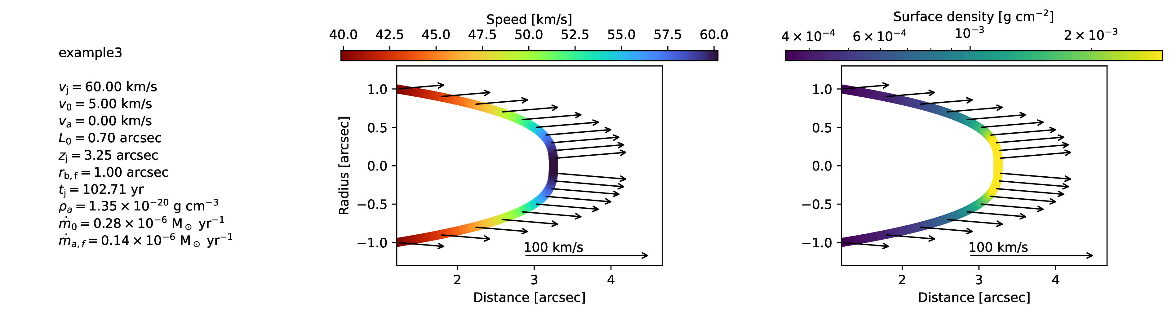
Bowshock model. This figure will be generate for each bowshock included in the cube.

Plots of the projected morphology and kinematics of the bowshock

For each bowshock, a plot named bowshock_projected_<n>.jpg will be generated showing the projected morphology and kinematics of the bowshock shell. On the upper left panel, the input parameters are listed, where i is the inclination angle of the bowshock symmetry axis with the line-of-sight and vsys is the systemic velocity of the source.

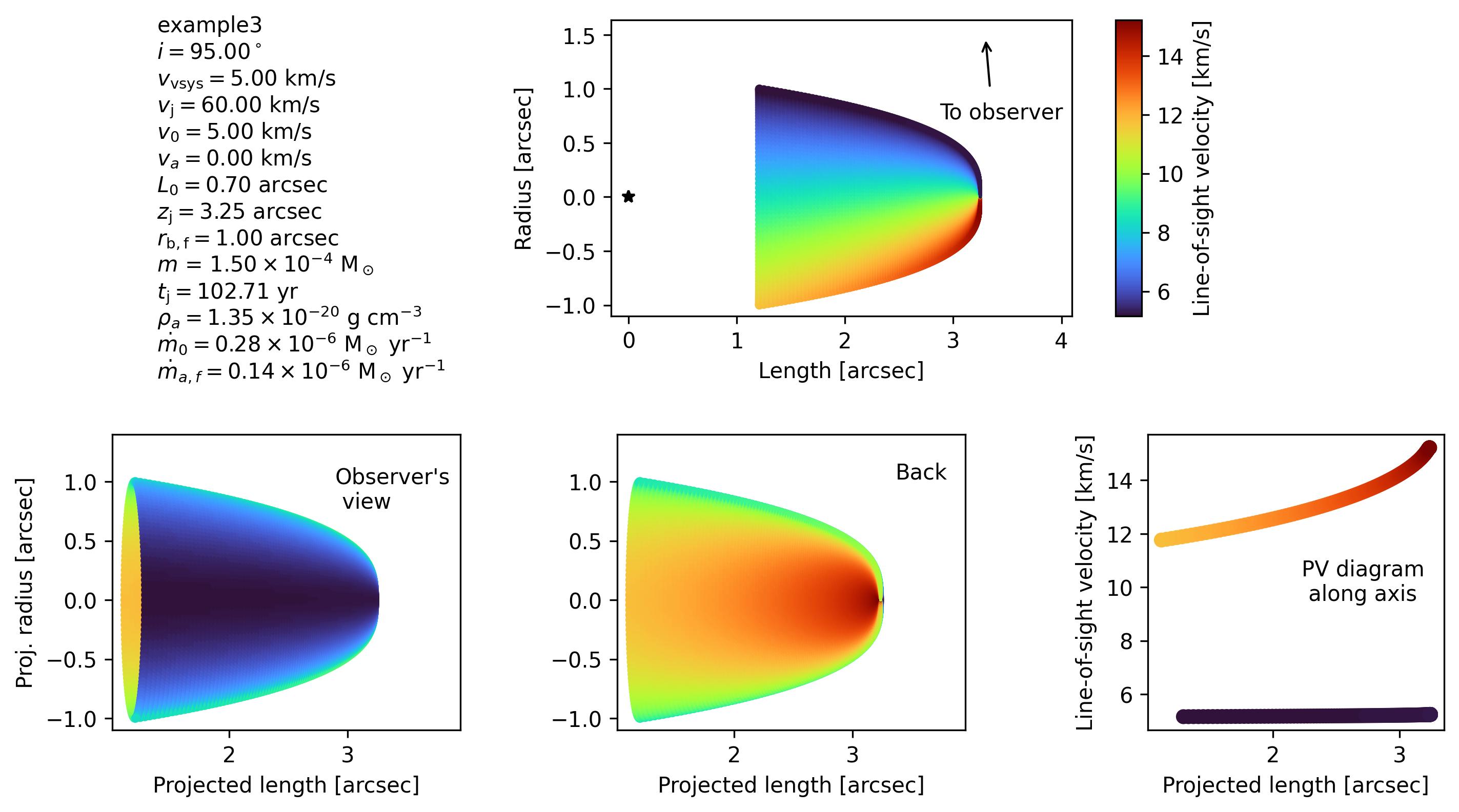
Projection of bowshock model. This figure will be generate for each bowshock included in the cube.

Plots of the channel maps

A plot with a selection of channel maps, named bowshock_cube_<cubename>.pdf, will be generated.

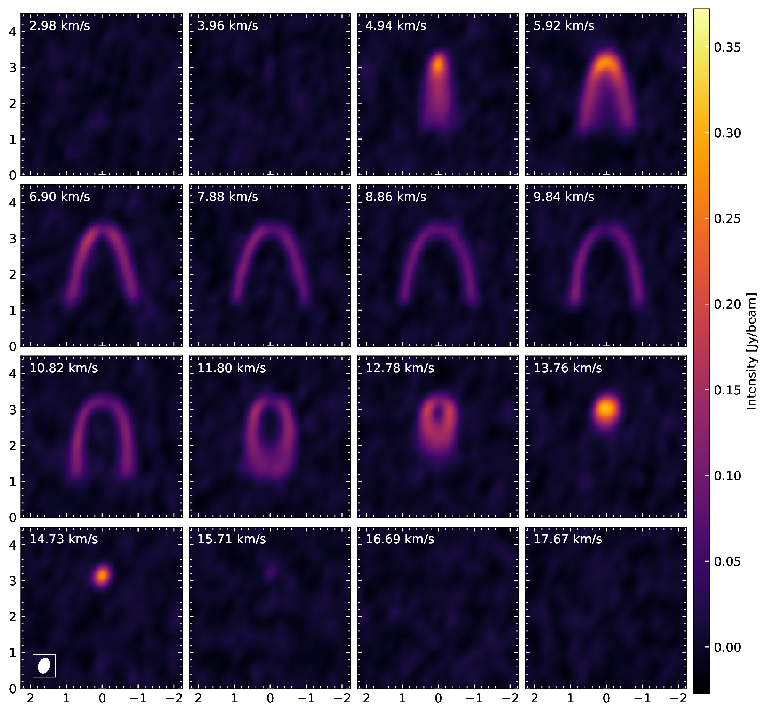
Channel maps of the bowshock model.

Plot of the moments and position velocity diagrams

If specified in the input parameter outcubes (see input file parameters section), a plot with the moments and position velocity diagram, named momentsandpv_and_params_<cubename>.pdf, will be generated.

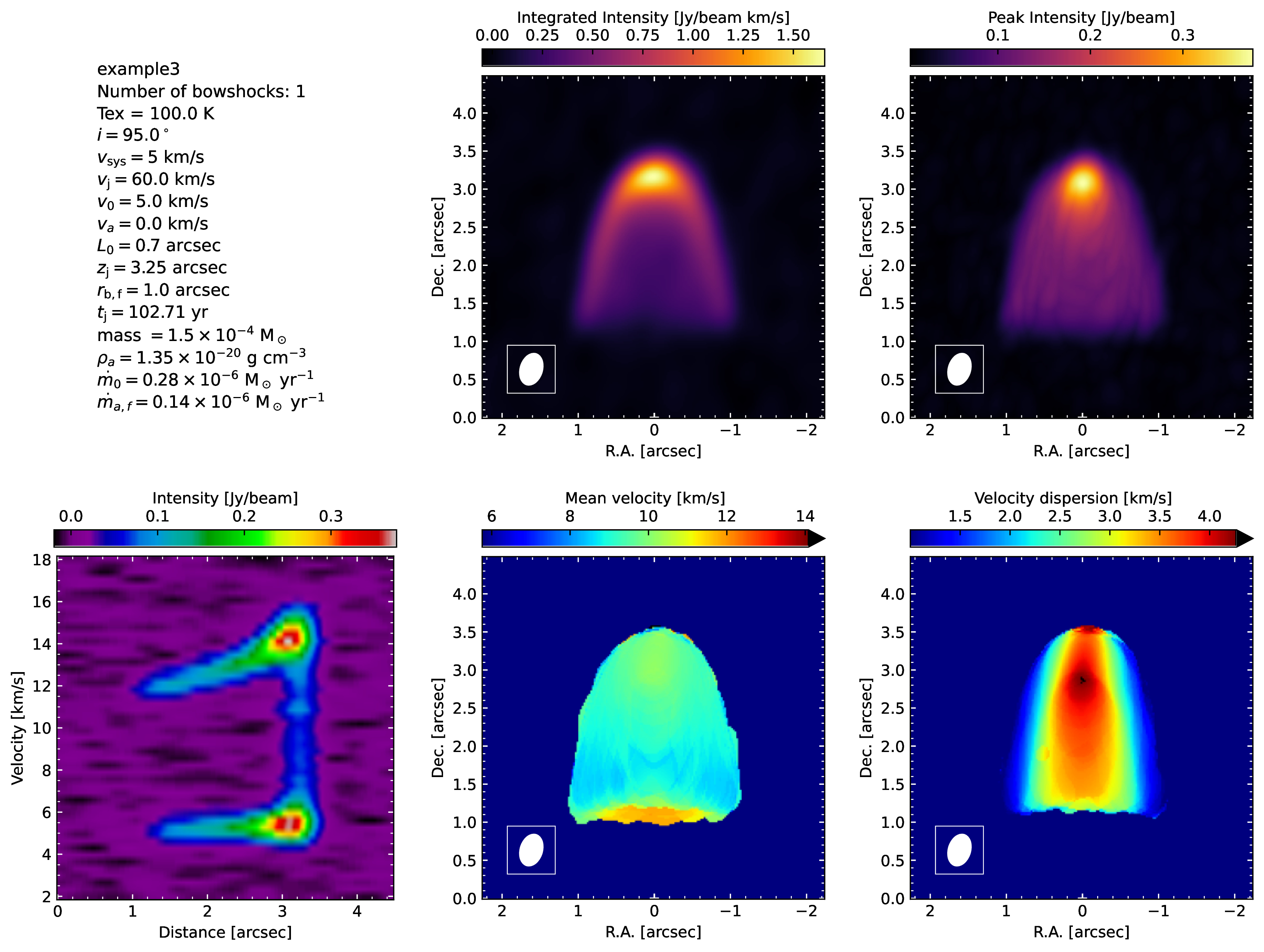
Moments and position-velocity diagram of the spectral cube.

Fits files

The cubes in fits files format will be saved in models/<modelname>/fits, and they can be open with casaviewer, CARTA, or ds9.

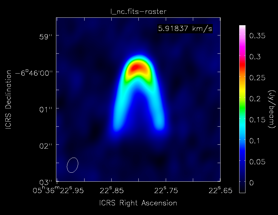
Channel map visualized with casaviewer.

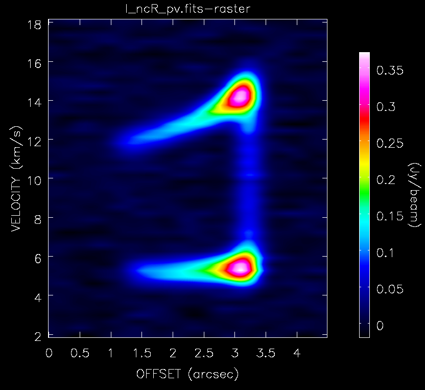
Position-Velocity diagram visualized with casaviewer.